The index and match formula is an advanced lookup which has many advantages over vlookups. It gives users the flexibility to combine horizontal and vertical matches as well as lookup multiple column or row criteria. Users also gain the ability to lookup columns to the left or rows above the criteria range.

The index and match formula may seem tricky at first, but this post aims to break down the two components and enable you to use it with confidence.

Syntax

• =INDEX(array,row_num,[column_num])

array: a collection of items that can be text or numbers in a column or row, or multiple columns and/ or rows
row_num: the number of the row of which to return a value from
column_num: the number of the column from which to return a value from

Imagine the array as a grid in the game battleship, with the row number and column number being your X and Y axis. If the array is only one row or one column then that value would be 1.

• =MATCH(lookup_value,lookup_array,[match_type])

lookup_value: this is the value that you are searching for
lookup_array: this is the row or column range that you are searching in
match_type: this is specifying whether you need an exact match (in most cases this will be true and should specify ‘0’ for an exact match)

The match formula returns the numerical value the row (left to right) or column (top to bottom) which corresponds to the lookup value.

Combining INDEX and MATCH

• =INDEX(array,MATCH(lookup_value,lookup_array,[match_type]),MATCH(lookup_value,lookup_array,[match_type]))

Explanation

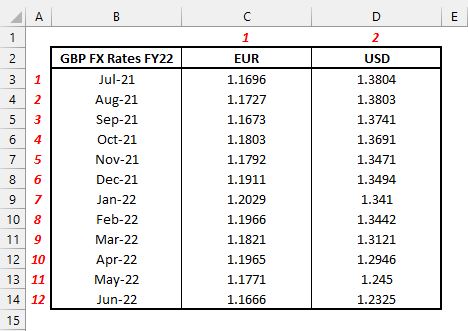
To help illustrate the argument within this formula consider the table below which features the foreign exchange rate against GBP for the financial year or a company. The array within the index formula relates to the table of values of the exchange rates depicted by the range C3:D14.

Remember the original index syntax earlier which asked for an array followed by a row number and column number. Instead of having static values they are now replaced with the match formula.

Instead of stating the row and column number of the array, we could simply ask Excel to reference them by matching the date and currency which we specify.

The formula would be written as below.

In other words, if we were to re-write the formula above and replace the match formula with the numerical values they are referencing for the row and column lookups, it would be as follows:

• =INDEX(C3:D14,2,1)

Where 2 is the row number reference, and 1 is the column number reference.

Usages

Use index and match functions as a replacement for vlookups. This avoids having to re-specify row numbers on vlookups when columns are inserted between the criteria and lookup range.

Return values based on a horizontal and vertical match in a table. This allows you to return a value from a table based on matching criteria from a row and column heading.

Return value based on multiple row or column criteria. Additional row or column criteria allows you greater flexibility with how you store and reference data.

Index and Match with multiple criteria

The index and match formula can be re-written easily to allow for a match on multiple criteria. This means changing the match element from a standard lookup to an array formula.

• =MATCH(lookup_value,lookup_array,[match_type])

Turns into.

• =MATCH(1,(criteria1=criteria_range1)*(criteria2=criteria_range2),[match_type])

As there is multiple criteria to satisfy in the lookup_array, the ‘1’ in the lookup_value is essentially asking to return the row number which satisfies all elements of the array.

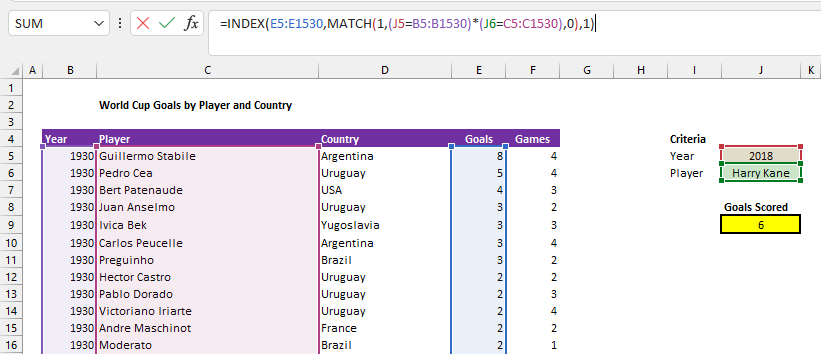
In the example below we nest the match formula within the index formula to find the row number within this table of World Cup goals by player and country.

• =INDEX(E5:E1530,MATCH(1,(J5=B5:B1530)*(J6=C5:C1530),0),1)

In this case it is returning the row number corresponding to ‘2018’ in column B and ‘Harry Kane’ in column C, which tells the index formula the correct row to pull the value from.

Limitations

Similar to the the vlookup, the index and match formula does have a weakness in the fact that it will return the first value which satisfies the criteria. The risk this poses is that there may be multiple values which satisfy the criteria and therefore it may not always retrieve the best fit. The index and match formula works best when there can only be one result for any combination of criteria such as the FX rates table above.

Summary

The index and match formula should be a staple in everyone’s Excel arsenal. The flexibility that is allows gives it many advantages over the vlookup formula, and makes it perfect for finance professionals for use in creating dashboards or retrieving data based on multiple criteria.